Putting the location-based hierarchy to the test

← All insights

The first three posts in this series each looked at one quality of a location-based emission factor. Part 1 found that every boundary coarser than the balancing area misstates inventories by 18% or more. Part 2 found that even the balancing area can be too coarse inside large markets, where using one market-wide factor instead of subregional factors misstated inventories by 19% or more on average in every simulated regional grid. Part 3 found that using last year’s emission factor data roughly doubles error, and leaves about a third of buildings off by more than 5%.

So each quality matters. But a hierarchy can’t just say that. Reporters often can’t get a factor that is best on every count, and the hierarchy has to tell them which quality to give up first. The proposed hierarchy explicitly ranks three qualities: spatial granularity first, then temporal granularity, then whether the factor reflects consumed or produced electricity (its type). It doesn’t list a factor’s vintage (whether it describes the reporting year or a prior year) as a ranked quality. But the proposal allows prior-year factors only when reporting-year data isn’t available, which implicitly ranks vintage first: any reporting-year factor, however coarse, comes before any prior-year factor.

In practice, for example, an annual-average factor at the operational grid boundary would be prioritized over an hourly factor at the national boundary, because spatial boundary is ordered before temporal granularity in the hierarchy.

But is this proposed ordering supported by the best available science? One simple test is that any ordering should generally improve inventory accuracy and relevance as you move up the hierarchy. This post asks whether the proposed ordering passes that test, what ordering the data supports instead, and whether the difference matters for the datasets reporters actually use.

How the proposed ordering was reached

The proposed consultation ordering reflected expert judgment about when each quality matters most. That judgment rests on a few general considerations:

• Type matters more where imports or storage supply a large share of the electricity a grid consumes.
• Spatial granularity matters more where generating resources are unevenly spread and transmission is constrained.
• Temporal granularity matters more where variable renewables make up a large share of supply and emission rates swing widely across the day or the seasons.
• The qualities interact. Production-based factors only reasonably approximate consumed emissions at boundaries broad enough that little power crosses them. Storage matters most at hourly resolution. On a small island grid, every boundary may be the same one.

These considerations resulted in the proposed hierarchy, but at the time, there was no analysis available to comprehensively or quantitatively evaluate all of these tradeoffs. This is the gap that this analysis seeks to fill.

How I tested it

I calculated inventories for every combination of the four qualities in the hierarchy: boundary, type (consumed or produced), vintage (reporting year or prior year) and time resolution (hourly, monthly or annual), with prior-year factors used only as annual averages, as the proposal requires. This means that for each building, I calculated 24 different 2025 emissions inventories, each using an emission factor from a different tier. I measured each one’s average error against the benchmark, an hourly, consumption-based balancing area factor for the reporting year, and then ranked the tiers from lowest to highest error to see which ordering of the four qualities the results support.

Figure 1 shows the results for the boundaries in the proposed hierarchy, plus a national average for reference.

Operational grid subregions aren’t included, because subregional factors are only available for the case studies in Part 2. Details are in the methods post.

What the full ranking shows

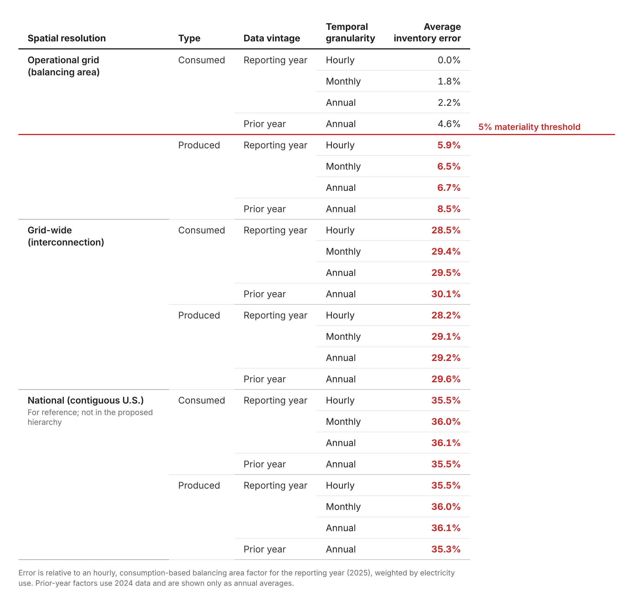
Three things stand out. First, location dominates. Every balancing area tier beats every grid-wide tier, and every grid-wide tier misses by 28% or more. Spatial granularity belongs first.

Second, within the balancing area, the results follow a clean order: type, then vintage, then time resolution. Every consumption-based tier beats every production-based tier. Within each type, every reporting-year factor beats the prior-year factor. And within the reporting year, hourly beats monthly, which beats annual. Only the consumption-based tiers fall below the 5% threshold.

Third, at a wide enough spatial boundary, the order of the other qualities stops mattering as much. This partially has to do with interactions between the criteria at a boundary this wide. At the interconnection, a production-based factor slightly beats a consumption-based one, because little power crosses a boundary that large. Nationally, prior-year factors happen to edge out reporting-year ones.

The proposed ordering, with temporal granularity ahead of type, doesn’t fit these results. It would place an hourly production-based balancing area factor (5.9%) ahead of an annual consumption-based one (2.2%).

What ranking the evidence supports

Put together, the results support this order:

1. Spatial granularity
2. Type (consumed over produced)
3. Vintage (reporting year over prior year)
4. Temporal granularity

Each step down this order adds error. Compared with the proposed ordering, two things change: vintage moves from first, where the proposal’s rule for older data implicitly puts it, to third, and type moves above temporal granularity.

The case for ranking vintage first

The results of this analysis alone would suggest ordering vintage third in the hierarchy. But there is a strong principles-based case for ranking it first.

The GHG Protocol’s decision-making criteria rank its accounting and reporting principles near the top, right after scientific integrity (Governance Overview, Annex A). One of those principles is relevance: an inventory should appropriately reflect the company’s emissions and serve the decision-making needs of its users. A location-based inventory is meant to describe the grid a company actually drew from in the year it used the electricity. A factor from a different year describes a different grid, however finely it is resolved in space or time. Accuracy is one of the same principles, and the criteria acknowledge that options can trade off between them. Ranking vintage third favors accuracy as measured here; ranking it first favors relevance.

There are also reasons to be cautious about letting the accuracy results decide. They come from one country, one year and one set of datasets, and it isn’t clear they generalize. A global ranking probably shouldn’t rest on them alone. And the accuracy cost of stale data is likely to grow. As the energy transition accelerates and grids change faster from one year to the next, last year’s grid becomes a worse stand-in for this year’s, so the accuracy argument increasingly points toward vintage first as well.

Timely factors also serve the next criterion in the hierarchy: supporting decision making that drives ambitious climate action. A company using current grid data sees the effect of grid decarbonization, and of its own choices about where and when it uses electricity, in the year they happen rather than a year or more later.

The theoretical tradeoff is real. Ranking vintage first means preferring a coarse current factor over a granular lagged one, even when the lagged one is more accurate: a reporting-year national factor misses by about 36%, while a prior-year consumption-based balancing area factor misses by 4.6%. However, as the next section shows, these theoretical tradeoffs may matter less in practice.

Does the ranking matter in practice?

A ranking only changes outcomes when real datasets force a tradeoff between qualities. In practice, few combinations of qualities are actually available. Figure 2 maps the datasets that are currently available to reporters in the U.S. onto every tier of the hierarchy: of the 24 tiers in the hierarchy, only five have a dataset. (Singularity, where I work, publishes the Grid Carbon API and the Open Grid Emissions dataset, and built the public dashboard that publishes MISO’s local resource zone factors.)

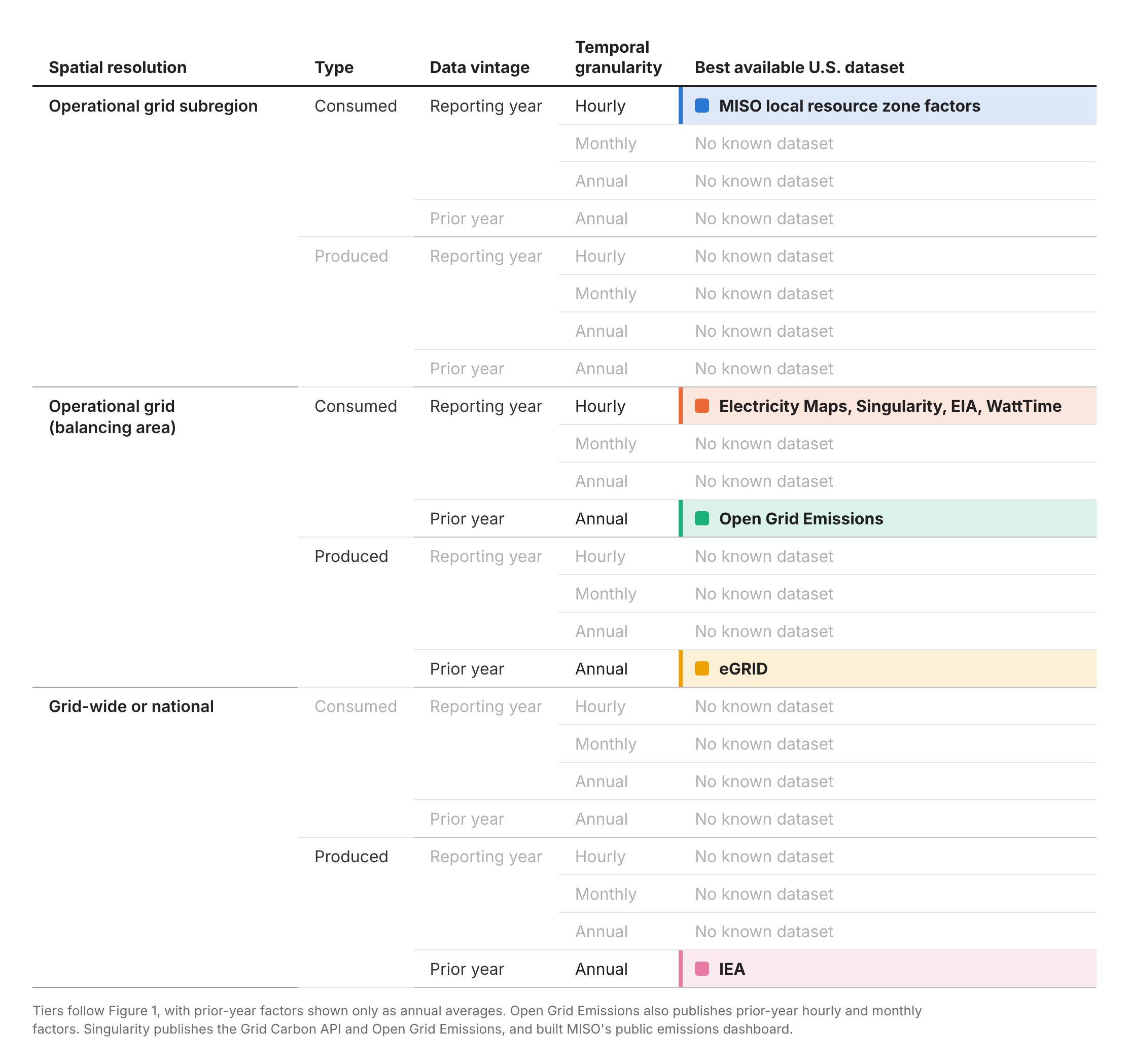
That sparsity is what makes the ordering question mostly academic in the U.S. today. The datasets that are best on one quality tend to be best on all of them: the most spatially granular datasets are also hourly, consumption-based and current, while the coarse ones are annual, production-based and a year or more old. Figure 3 ranks the same five datasets under three orderings: the public consultation proposal; the same order with type and temporal switched; and the error-minimizing order from Figure 1. The columns are rearranged to match each one. The datasets come out in the same order every time.

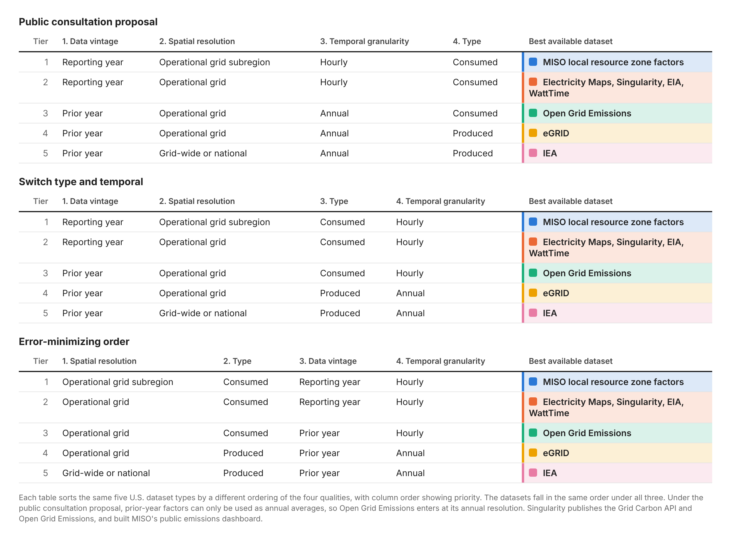
What matters more in practice is that free, consumption-based, hourly data at the balancing area level already exists for the whole country. A hierarchy that points reporters toward it, and away from coarse defaults, captures most of the accuracy available.

What the series adds up to

This series set out to answer one question: what makes a good location-based emission factor? Four answers came out of the analysis:

1. Location matters most. Every boundary coarser than the balancing area misstates inventories by 18% or more on average (Part 1).
2. The balancing area isn’t always fine enough. Inside large markets, a single market-wide factor misstates inventories by 19% or more on average compared with operational grid subregion factors, in every simulated regional grid (Part 2).
3. Vintage beats temporal resolution. Prior-year data roughly doubles error, and prior-year hourly factors add almost nothing over an annual average (Part 3).
4. Type ranks above temporal resolution. Ranking consumed over produced factors before temporal resolution minimizes error at each step, and by error alone, type ranks above vintage too (this post).

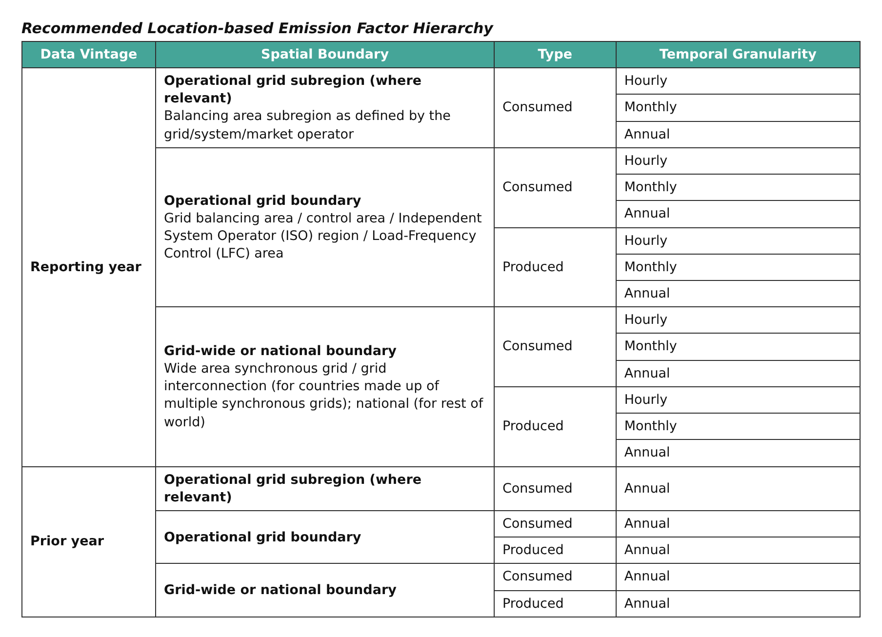
My recommendation for the GHG Protocol’s revision is therefore to rank vintage first, to best align with the accounting principles; keep an operational grid subregion (“local”) tier at the top of the hierarchy where it is relevant; rank emission factor type ahead of temporal granularity; and allow only annual factors when using prior-year data.

The data, assumptions and limitations behind all four parts are in the methods post.