This is Part 3 of a four-part series, What makes a good location-based emission factor?, which uses new analysis to answer open questions about the emission factor hierarchy proposed in the GHG Protocol’s revision of its Scope 2 Guidance.
- How much does location matter in location-based accounting?
- How local should location-based accounting be?
- How current do emission factors need to be? (this post)
- Putting the location-based hierarchy to the test
Many location-based emission factor datasets aren’t published in time for the inventories that use them. EPA’s eGRID, the most widely used U.S. dataset, is published about a year after the year it covers, and international datasets such as the IEA’s often arrive two or more years late. A company closing its 2025 inventory in early 2026 is usually multiplying 2025 electricity use by a factor that describes the grid in 2024, or earlier.
This lag has been normal for so long that it rarely draws attention, but it came up clearly in the GHG Protocol’s public consultation on the Scope 2 revision. Among respondents who gave low support to the proposed requirement to use the most precise emission factor available, 52% raised concerns about how often hourly and monthly datasets are updated, or how well they represent current conditions (Summary of Feedback, p. 33).
The proposed revision addresses older data, but only in passing. Its emission factor hierarchy ranks factors on three qualities: spatial granularity, temporal granularity, and whether the factor reflects consumed or produced electricity. Separately, it proposes that “where only emission factors older than the reporting period are accessible, the most recent accessible annual emission factors shall be used” (emphasis added). Read literally, that rule ranks vintage first without saying so: a prior-year factor is allowed only when no reporting-year factor is accessible at all.
I’d argue that a factor’s vintage, meaning the year it represents, matters just as much to its quality, and should be ranked alongside the other three qualities.
This post tests that idea. It asks how much vintage actually matters, why prior-year factors should only be used as annual averages, and where vintage belongs in the hierarchy.
Why data lag matters
Why would a year or two matter? Because operating conditions change from year to year, and many grids are changing quickly as the energy transition continues. In MISO, for example, the generation-based emission rate has moved by roughly 7% from one year to the next in recent years. A factor that is a year old can be off by enough to affect materiality before any question of spatial or temporal granularity comes up.
Lag also delays the signal location-based accounting is supposed to send to decision-makers. If a company’s reported emissions reflect the grid as it was a year or more earlier, then grid decarbonization, or a grid getting dirtier, shows up in its inventory late. Anyone using those numbers to understand the effect of where and when they use electricity is looking in the rearview mirror.
The biggest consequence is less obvious. Most companies calculate their inventories in the first half of the year after the reporting year ends. If reporting-year factors aren’t available by then, and the hierarchy only allows prior-year data as an annual average, location-based accounting stays an annual method in practice, even with hourly and monthly factors at the top of the hierarchy.
So the question of how current a factor needs to be is tied up with how granular it can be. That is what the analysis below tries to untangle.
How I tested it
To isolate vintage, I used the same setup as the earlier posts (details in the methods post). The benchmark is each building’s 2025 emissions calculated with an hourly, consumption-based factor for its own balancing area, built from 2025 EIA-930 data. I then recalculated the same 2025 electricity use with 2024 emission factors and compared the two.
I tested prior-year factors at three temporal resolutions: hourly, monthly and annual. For comparison, I also calculated reporting-year monthly and annual factors.
Location and type stay fixed throughout: every factor is a balancing area, consumption-based factor. Any difference from the benchmark comes only from the age of the data and its time resolution. As in Parts 1 and 2, error is the absolute difference in each building’s annual emissions, weighted by electricity use, and I treat 5% as the threshold for a material error.
What a prior-year vintage costs
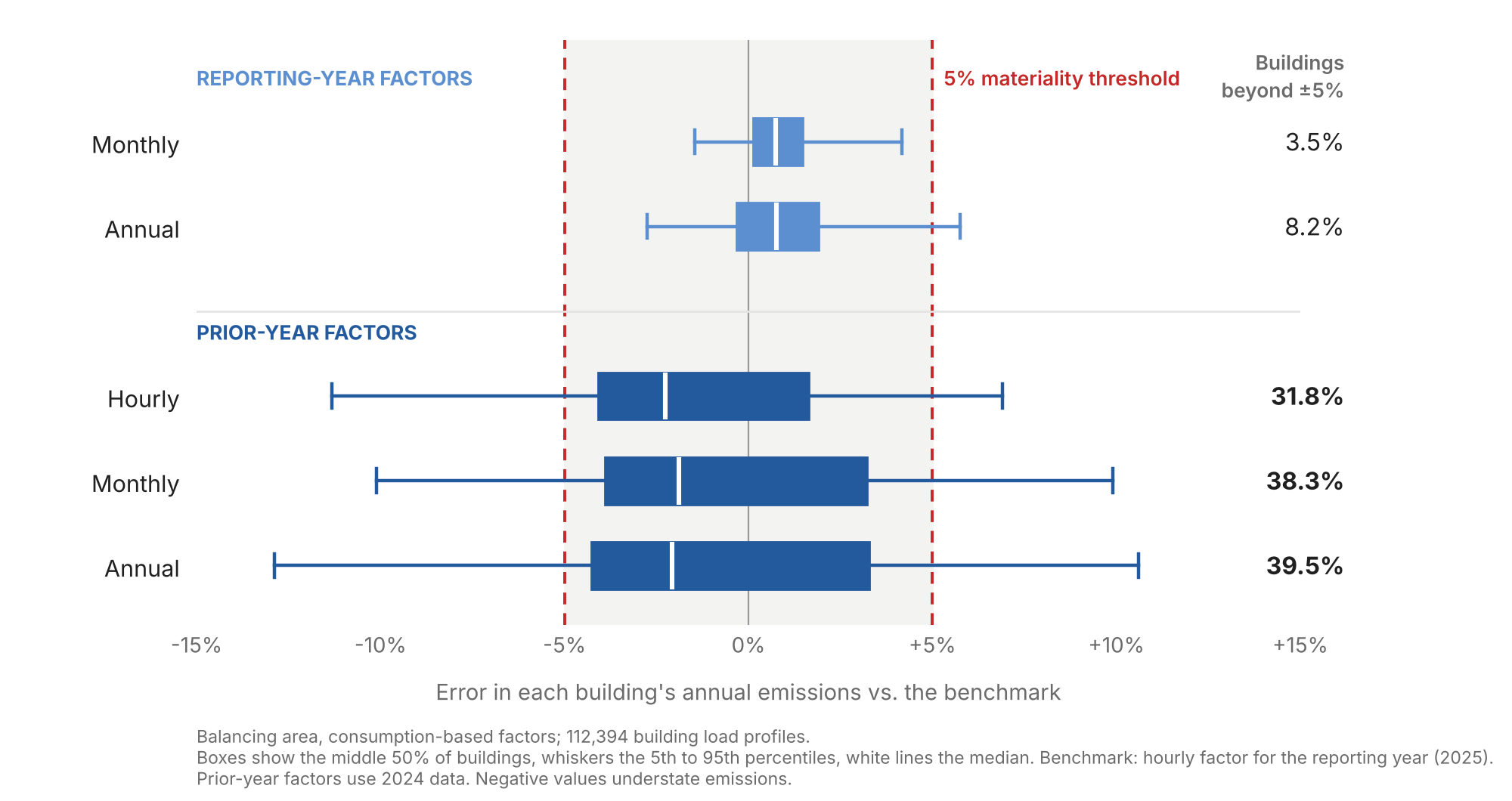
Using last year’s data roughly doubles the error. With reporting-year data, monthly and annual factors land within about 2% of the benchmark on average. With prior-year data, every resolution lands between 4.3% and 4.6%.
A skeptic could look at those averages and conclude that vintage doesn’t matter much. Every prior-year option is still under the 5% threshold on average. But averages hide the spread. With prior-year factors, between 32% and 40% of buildings have errors above 5%. With reporting-year factors, the share is 0% for hourly, 3.5% for monthly and 8.2% for annual. A company doesn’t report the population average; it reports its own inventory. With prior-year data, roughly one in three would be off by more than 5%.
Prior-year hourly data buys almost nothing
If prior-year data is all that’s available, does it help to use it at a finer resolution? Barely. Prior-year hourly factors produce 4.3% error, compared with 4.6% for prior-year annual factors, a gap of 0.3 percentage points. The share of buildings above 5% tells the same story: 32% for hourly and 40% for annual.
Why so little? Hourly factors are valuable because they capture what the grid did in the hours a building used electricity. Last year’s hours don’t carry that information. Weather, wind and solar output, outages and fuel prices make each hour’s emission rate specific to its year. Matching 2 p.m. on March 3, 2025 with 2 p.m. on March 3, 2024 also pairs a Monday with a Sunday. Prior-year hourly factors look precise, but much of that precision is false.
This supports limiting prior-year factors to annual averages, as the proposed hierarchy does. The added complexity of prior-year hourly factors buys very little accuracy. But it also confirms the concern from earlier: if prior-year data is all companies can get when they report, location-based accounting stays annual in practice.
Where should vintage rank?
The proposed hierarchy doesn’t rank vintage explicitly. I think it should, and there is a principled case for ranking it first. Under the GHG Protocol’s principle of relevance, a location-based factor should describe the grid a company actually drew from. A factor from a different year describes a different grid, however finely it is resolved in space or time. Temporal granularity only adds information if the hours being matched are the right hours.
The error data points the same way. Reporting-year annual factors (2.2%) beat prior-year hourly factors (4.3%), and reporting-year monthly factors (1.8%) beat every prior-year option. Measured by error, vintage matters more than temporal resolution: a reporting-year annual factor is a better choice than a prior-year hourly one.
When only prior-year data is available, the opposite holds. As the previous section showed, finer prior-year resolution adds complexity without meaningfully improving accuracy, so an annual average is enough.
Most of the accuracy comes from using reporting-year data at all. That suggests the most useful thing for location-based accounting may not be a better ranking rule, but making reporting-year data available, and trustworthy, by the time companies report.
A note on data quality: there is a separate question of whether timely data is as accurate as lagged data, since part of what makes some datasets lag is survey-based data collection and quality assurance. This series takes reporting-year data at face value; a separate post will test it.
How vintage should rank against type and spatial granularity is a harder question, and the answer isn’t the same across every pair of qualities. Part 4 puts the pieces together: how all four qualities should be ranked against each other, and whether the ranking changes results in practice.
Next: Part 4, Putting the location-based hierarchy to the test