Tools
The data and methodologies behind Singularity’s emissions accounting.
Whether you want to know how much a generator actually emitted, the carbon intensity of the electricity delivered to a specific location, or the emissions impact of shifting load on the grid, Singularity has built the data and methodologies to answer those questions. Every methodology is documented, transparent, and built to hold up to scrutiny.
Open source · Free to use
Open Grid Emissions
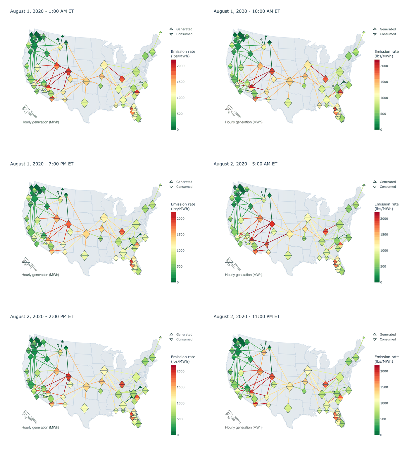
Built on the same methodology as EPA’s eGRID dataset, OGE is the next generation of U.S. grid and emissions data, built for the needs of today’s analysts, researchers, and carbon accountants. Covering 2005–2025, it contains annual, monthly, and hourly-resolution data for all generators in the U.S., as well as regional, consumption-based emissions factors for location-based Scope 2 accounting. This free, open-source dataset represents the most comprehensive, accurate, and granular emissions and generation data for the U.S. power sector.
Regions: All U.S. balancing authority areas
Granularity: Annual, monthly, hourly (hourly available 2019–present only)
Emissions type: Generated and consumed
Open-source, transparently documented, and peer-reviewed.
- Generator-specific data (not only plant-level aggregations)
- Hourly and monthly data (not only annual)
- Consumption-based emissions factors (reflecting imports/exports)
- Published months before eGRID is available
Real-time · Free trial available
Grid Carbon API
The Grid Carbon API delivers real-time, historical, and forecasted carbon intensity data across all U.S. balancing authorities and parts of Canada: generated, consumed, and marginal emissions, all built on the same methodology as our other tools. Developers, enterprises, and energy practitioners use it for Scope 2 reporting, 24/7 clean energy tracking, and any application that needs current, traceable emissions data.
Multiple use cases, one API
Generated, consumed, and marginal carbon intensity for Scope 1, Scope 2, and avoided-emissions accounting respectively (marginal covers ISONE, MISO, SPP, and PJM). Query CO2 or CO2e weighted by global warming potential. Fuel mix data supports hourly carbon-free energy (CFE) percentage for 24/7 matching.
Data within hours, not years
Datasets like OGE and eGRID are built for retrospective accuracy but are published on a one-year lag. The Grid Carbon API fills the gap in between: near-real-time data, current within hours to days, plus forecasts up to 24 hours ahead.
Free for academic research
Verified researchers with a .edu email get access to the same real-time API, at no cost, renewed annually. Need historical data instead? That’s what Open Grid Emissions is for. Apply for academic access →
Residual mix, approximated
Market-based Scope 2 needs an emission rate for power not covered by a REC or PPA. Without it, you risk double-counting clean energy someone else claimed. A complete residual mix would require every REC and contract on record, so we provide a fossil-only rate that assumes all carbon-free generation has already been claimed, including for unspecified purchases and imports.
Utility & grid operator deployment
GRETA: Generator Real-Time Emissions Assignment
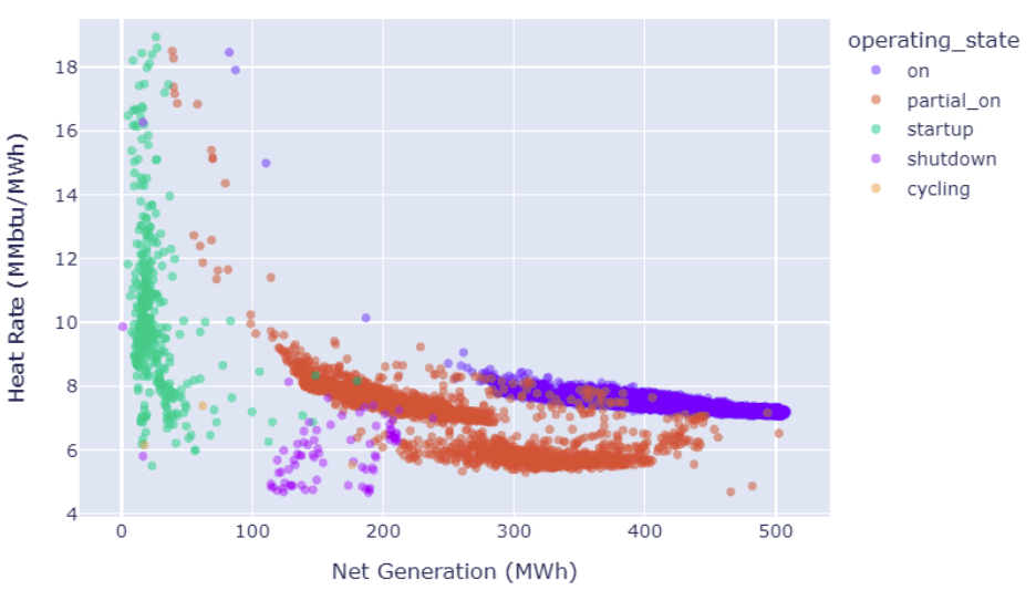
GRETA (Generator REal-Time emissions Assignment) estimates the direct, Scope 1 stack emissions of a power plant in real time, using only its net generation output. It exists for the use cases that static, annual emission factors can’t serve: real-time market operations, carbon pricing, and 24/7 clean energy accounting all need emissions data that reflects what a generator is doing right now, not what it did on average last year. A generator’s heat rate shifts hour to hour with fuel switching, operating state, and ambient conditions, and GRETA models that variation directly instead of assuming a fixed rate. The result is interval-level emissions (CO2, CH4, N2O, and CO2e, in lb and lb/MWh) at 5-minute or hourly resolution.
A model for every generator behavior
GRETA uses four models per generator: a heat rate curve fit by operating state and season, an operating-state classifier (off, starting, fully on, or partially on), a fuel-type model for units that switch or co-fire, and a CHP model that splits fuel between electricity and heat. Each captures a different way real emissions diverge from a flat annual average.
Built on public data
GRETA trains on EPA CEMS readings and EIA Forms 860 and 923, so there’s no proprietary black box and nothing extra to collect. The only required input at run time is a generator’s net generation output (MW). If a fuel-switching event is known, you can specify it, but GRETA’s fuel-type model works without it.
Benchmarked against measured emissions
When benchmarked against actual, measured emissions data from continuous emissions monitoring systems (CEMS), GRETA is consistently the most accurate method to estimate a generator’s actual, hourly emissions. It can substantially reduce emissions accounting error compared to traditional methods of estimating generator emissions, like static annual emissions factors from eGRID.
Trusted across the grid
GRETA is in active use at MISO, SPP, Southern Company, and Arizona Public Service. These utilities and grid operators rely on it for real-time emissions tracking, market monitoring, and clean energy program administration.
Grid operator deployment · Sub-regional granularity
CarbonFlow
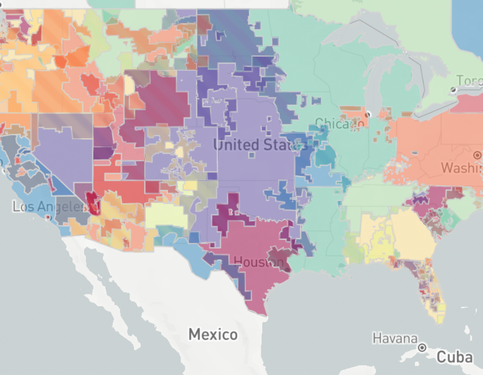
CarbonFlow traces the physical path that electricity takes across the transmission grid, along with the emissions that travel with it, from the generators that produced the power to the specific locations that consumed it. Regional or balancing-authority averages can’t capture how emission rates vary within a region; CarbonFlow can, calculating consumed emission rates down to the county, city, or individual transmission node.
How it works: power flow tracing
Power flow tracing is a standard power systems technique for determining how individual generators contribute to flows on transmission lines and ultimately to specific loads. CarbonFlow applies the same technique to emissions: once a generator’s emissions are known, tracing its power flow attaches those emissions to the physical path they take to the load being served.
Granular down to any local region, node, or substation
It uses the same math behind regional, consumption-based emission rates, extended with a transmission network model to reach any boundary you define: a node, a substation, a county, or any custom area, rather than stopping at a balancing-authority average.
Localized insights
In large ISO/RTO regions like MISO, subregional emission rates vary substantially from footprint-level averages, especially where transmission congestion limits how power flows. CarbonFlow surfaces that variation for Scope 2 accounting, clean energy deliverability verification, and policy analysis that needs to know where emissions are delivered, not just where they’re generated.
Traces power flows, not electrons
A common objection: individual electrons can’t be tracked through a grid. CarbonFlow doesn’t track electrons. It traces power flows, the physical quantity of how much power moves across each line, a method used for decades to allocate costs, losses, and other attributes to sources and sinks. Emissions are another attribute carried along that same flow.
Grid operator deployment · Nodal · 5-minute resolution
Locational Marginal Emissions (LME)
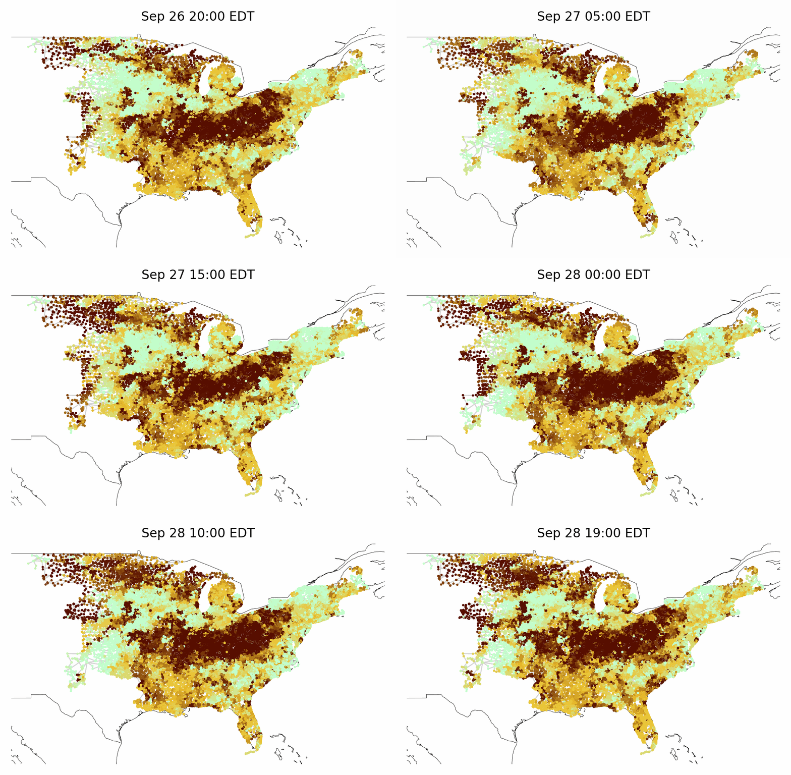
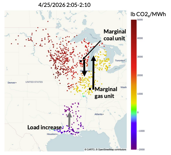
Locational Marginal Emissions (LME) describe how system-wide emissions would change in response to a small shift in electricity demand at a specific location on the grid. An average emission rate can’t capture this: the same load increase can raise emissions in one part of the system and lower them in another, depending on which generators are actually on the margin and how transmission constraints route the resulting redispatch. Working with MISO, we calculate LMEs directly from the security-constrained economic dispatch (SCED) engine behind every market interval, using GRETA’s dynamic heat rate curves rather than static annual emission factors, and publish the results at every commercial pricing node, every five minutes.
Granular in space and time
LME values cover every commercial pricing node in MISO’s footprint at five-minute resolution, granular enough to show how emissions impacts vary from location to location and hour to hour. The marginal unit changes from interval to interval, fuel types vary, and redispatch can be negative. These patterns are invisible in annual or hourly-average rates.
Accessible data exploration
The public LME dashboard links a map and timeseries view: track a single node across a full day, or see the entire footprint at a single moment, with a time slider connecting both. Alongside LME, the Locational Marginal Fuel (LMF) metric shows which fuel types are driving the value. CSV download and API access are available for programmatic use.
Transparent and trusted
LMEs are calculated directly from MISO’s actual market-clearing results, not estimates or assumptions, using a fully publicly documented methodology rather than black box approaches. Every calculation is also continuously validated against the market’s own prices and sensitivities before it’s published, so accuracy can be monitored and improved over time rather than taken on faith.
Best-in-class methodology
LME uses GRETA’s dynamic, unit-specific heat rate curves rather than a static annual factor, capturing how a generator’s efficiency shifts by output level, season, and operating state. The calculation incorporates MISO-specific innovations: reserve and transmission constraints, the constraint demand curve to distinguish binding constraints from violated ones, and a two-stage marginal-unit identification process validated against live operational data.
Singularity Energy
Running a clean energy program?
These tools are built on the same carbon accounting work Singularity does inside utilities and grid operators. If you need that methodology applied to your program data (customer attribution, hourly reporting, compliance documentation), that’s what the platform is built for.
Get a demo →Large C&I buyer? If you want this level of data from your utility (hourly by source, matched to your actual load), ask your utility about the platform. The Georgia Power deployment with Google is an example of what that looks like.