How local should location-based accounting be?

← All insights

In Part 1, I found that spatially coarse emission factors introduce large errors into location-based Scope 2 inventories. Every boundary coarser than the operational grid boundary (balancing areas) misstated the average building’s inventory by 18% or more, well above the GHG Protocol’s 5% materiality threshold. That supports putting the operational grid boundary, which in the U.S. generally means the balancing area, near the top of the emission factor hierarchy.

But balancing areas are not all alike. Some cover a single metropolitan area, like the Los Angeles Department of Water and Power or Seattle City Light. Others are regional markets that span many states: MISO’s footprint covers parts of 15 states, and SPP now operates across two separate interconnections. As regional markets expand, some of these footprints keep getting larger.

So is the operational grid boundary always granular enough? Or does a single factor for a footprint the size of MISO hide the same kind of variation that Part 1 found inside interconnections? It is also a live debate. In the GHG Protocol’s public consultation, one of the most common concerns among respondents who gave low support to the requirement to use the most precise factor was that the proposed “local” boundary is too narrow. This post asks whether subregional factors change inventories enough to justify a tier above the operational grid boundary, and how that tier could be defined so these concerns are addressed.

One balancing area, many grids

Most of today’s large regional markets were built by combining utilities that once operated as their own balancing areas. When a utility joins a regional market, it hands dispatch over to the market operator, but its old footprint does not disappear. Market operators continue to use these areas, and others they define, for their own planning, reliability and settlement work. MISO, for example, divides its footprint into 10 “local resource zones” for resource adequacy planning, along with about 40 “local balancing authorities,” many of them once independent balancing areas. PJM organizes its footprint into transmission zones that trace back to its member utilities.

These subdivisions are not academic. The U.S. Energy Information Administration’s Hourly Electric Grid Monitor asks balancing areas to report demand for subregions within their footprint if they already calculate it “in the normal course of business.” Today, 10 of the roughly 60 U.S. balancing areas do, mostly the large regional markets (MISO, PJM, SPP, ERCOT, CAISO, NYISO and ISO New England) along with two Western utilities. In other words, the operators of the largest grids already define and use these subregions in their operations.

The proposed hierarchy anticipates this with a tier above the operational grid boundary, which it calls the “local boundary”: a subregion defined by a grid or market operator. Throughout this post I’ll refer to it as an operational grid subregion, which describes what it is more precisely. The question is whether using these subregions instead of the full balancing area footprint actually changes inventories by a material amount.

How I tested it

EIA does not publish emission factors below the balancing-area level, so I tested the value of operational grid subregions in two ways. First, I used real subregional factors from MISO, which publishes hourly consumption-based emission factors for multiple types of subregional boundaries. Second, I simulated large regional grids using EIA data, treating groups of neighboring balancing areas as if they were a single market and each member balancing area as one of its subregions.

Both cases use the same approach as Part 1: building-level inventories calculated with hourly, consumption-based factors, compared against a benchmark. Here, the benchmark is the inventory calculated with the subregion’s own factor, and the question is how much that inventory changes when the full regional footprint’s factor is used instead. The full methods are described in the companion methods post.

Case 1: MISO’s local resource zones

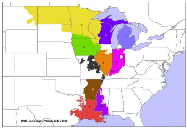
MISO publishes 2025 hourly consumption-based emission factors for each of its 10 local resource zones through its public consumed emissions dashboard. (Singularity built and operates this dashboard for MISO.) For buildings in each zone, I compared inventories calculated with the zone’s own factor to inventories calculated with the factor for MISO’s full footprint.

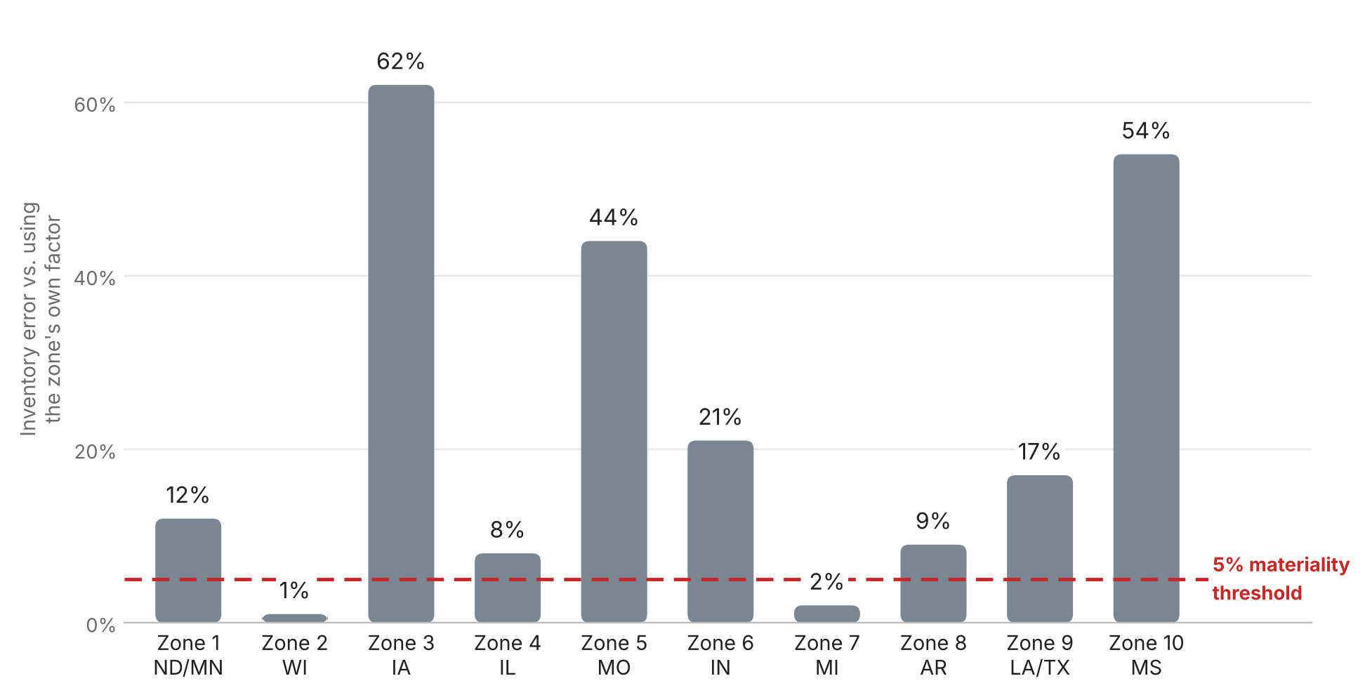
In 8 of MISO’s 10 zones, using the footprint-wide factor misstates the average building’s inventory by more than 5%. In three zones the error exceeds 40%: Missouri (44%), Mississippi (54%) and Iowa (62%). Only in Wisconsin and Michigan, where the zone’s consumption-based emission rate closely tracks MISO’s overall rate, does the footprint-wide factor stay within the materiality threshold.

These differences reflect real differences in how each part of MISO is supplied. Iowa (Zone 3), for example, gets a large share of its electricity from wind, while Missouri (Zone 5) relies more heavily on coal. A single footprint-wide factor averages these together and assigns every reporter in MISO the same rate, much as an interconnection-wide factor did in Part 1.

Case 2: simulated regional grids

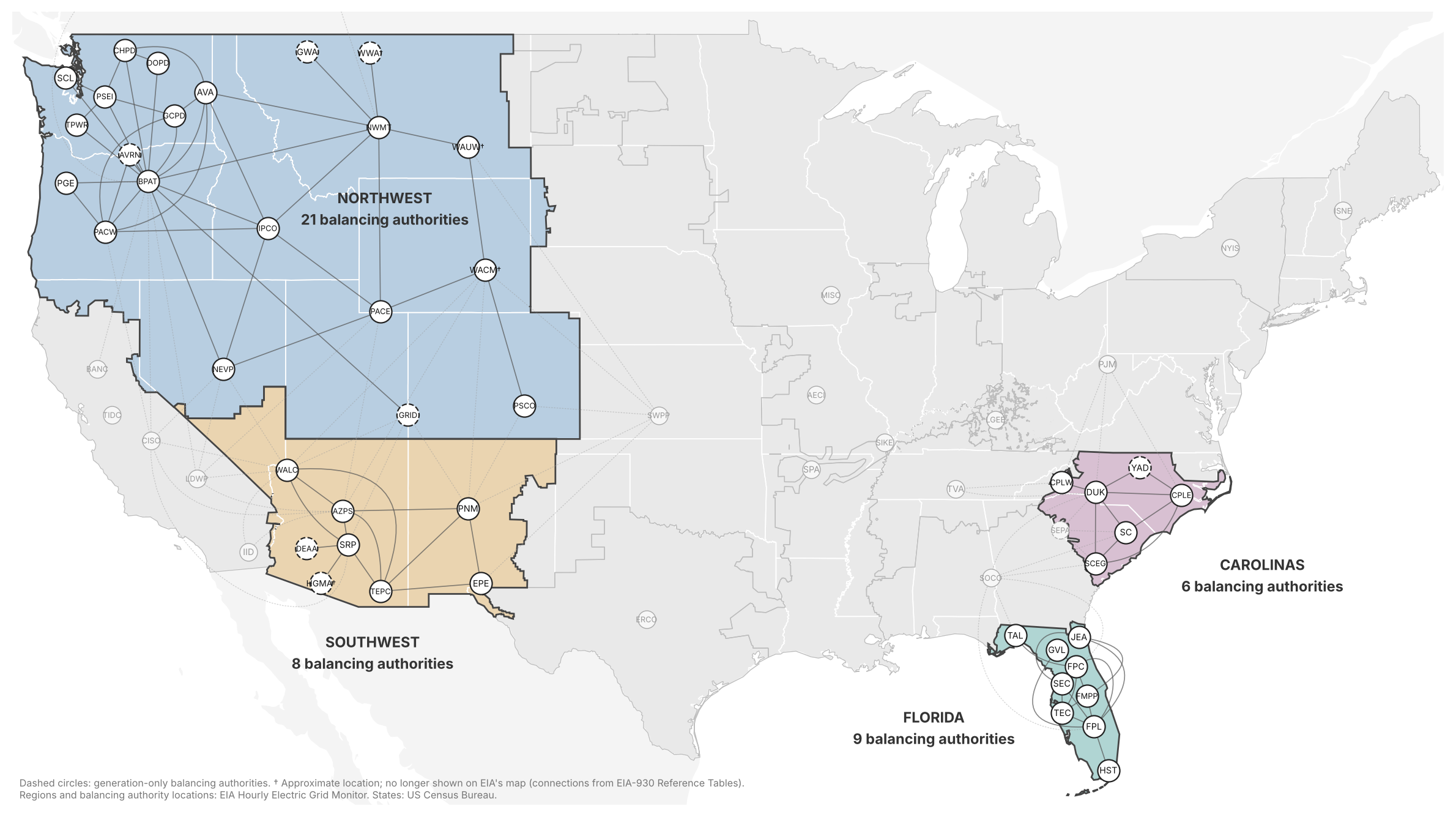
MISO is one market. To test whether its results generalize, I used regions defined by EIA that group neighboring balancing areas together, and treated each region as if it were a single regional market. Each member balancing area then plays the role of an operational grid subregion, much like the utilities that joined MISO or PJM. I tested four regions: the Southwest (8 balancing areas), the Carolinas (6), Florida (9) and the Northwest (21). The Northwest is a particularly relevant case. Many of its balancing areas are joining regional day-ahead markets, such as CAISO’s Extended Day-Ahead Market (EDAM) and SPP’s Markets+. They will remain separate balancing areas, but as more dispatch is coordinated across these larger footprints, it becomes more important to know what a single footprint-wide factor would miss.

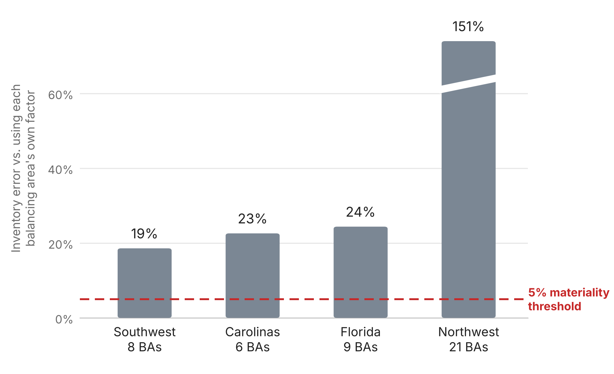
In every region, the region-wide factor introduces material error: 19% to 24% in the Southwest, the Carolinas and Florida, and 151% in the Northwest. These results line up with Part 1, where EIA regions introduced 18% error on average compared with balancing-area factors.

The Northwest stands out because of how much its members differ. While some balancing areas are coal-heavy, others are supplied almost entirely by hydropower, so their own emission rates are close to zero. This means that even small absolute differences from the regional emission rate result in large percentage errors.

Making a subregional tier work

Respondents who found the local boundary too narrow pointed out that power flows across interconnected grids rather than staying within small areas, and a few worried that narrow boundaries would make a company’s results depend on its proximity to legacy fossil plants or pockets of grid congestion (Summary of Feedback, p. 21). Others raised a comparability concern: if “local” can mean different things, reporters on the same grid could end up using different factors.

A well-defined tier can address these concerns.

First, consumption-based factors already account for power flowing in from the wider grid. A subregion’s consumption-based factor reflects the electricity its customers actually receive, including imports from the rest of the market, not just the output of the plants located inside it. This is also why the proposed hierarchy only offers consumption-based factors at the subregional tier: a production-based factor for a small area would indeed overweight nearby plants.

Second, the concerns about comparability are legitimate if “local” is left open to interpretation. A tier that allowed any city, county or zone drawn for any purpose would invite exactly the inconsistency and cherry-picking respondents described. However, the hierarchy defines this tier specifically as an officially defined, operationally relevant subregion of a grid. Thus, if paired with language that there could only be a single officially recognized set of subregional boundaries used for each operational grid, it mitigates these concerns.

Finally, the regions where such operational subregions even exist are pretty limited. As the EIA data shows, only a handful of large regional markets track subregional demand today. Most reporters, served by smaller balancing areas, would never encounter this tier.

What this means for hierarchy design

The results point to keeping a tier above the operational grid boundary, but defining it much more tightly than “local.” In large, regionalized grids like MISO, the operational grid boundary does not reflect the spatial variation that exists in the electricity delivered to each of these operational subregions. Removing the subregional tier in these grids would introduce large errors in location-based inventories.

A well-defined operational grid subregion tier would:

1. Apply only where it is relevant: inside large, regionalized operational grids that contain operationally distinct subregions. Most balancing areas would have no subregional tier at all.
2. Use boundaries the grid operator already defines: subregions the operator uses in the normal course of business for balancing, planning or reliability, such as MISO’s local resource zones or local balancing authorities. Arbitrary lines like cities or counties would not qualify.
3. Name one set of “official” subregions per grid: so that every reporter on that grid reads the tier the same way, the same principle that should apply to every tier of the hierarchy.
4. Use consumption-based factors only: so that subregional factors reflect power delivered from across the wider grid, not just nearby plants.

Defined this way, the tier keeps an important locational signal inside the largest markets, where it is most useful for decisions about where to site new load or clean resources, without opening the door to arbitrary or inconsistent boundaries.

So far, every comparison in this series has used emission factors for the same year as the electricity use being measured. In practice, many widely used datasets are published a year or more after the fact. Part 3 asks how much that lag matters, and where a factor’s vintage should rank in the hierarchy.

Next: Part 3, How current do emission factors need to be?